A Single-Cell Atlas of Radiation-Induced Lung Injury (RILI) at the Early Stage Post-FLASH and Conventional Dose Rate (CONV) Irradiation

Summary

Radiation therapy (RT) is essential for treating thoracic malignancies but often causes significant lung damage. FLASH-RT, an ultra-high dose rate irradiation technique, shows potential in reducing radiation-induced lung injury (RILI) while maintaining tumor control. However, the mechanisms underlying its benefits, particularly immune modulation, remain unclear. This study investigates the immune and cellular responses to FLASH-RT versus conventional dose rate (CONV) RT during the early phase of RILI. Using single-cell RNA sequencing (scRNA-seq), we pictured a dynamic landscape of the lung microenvironment during RILI within one week post-irradiation. Our analysis revealed that FLASH-RT induced a more immediate but transient cellular response, while CONV-RT caused sustained inflammation. FLASH irradiation significantly reduced neutrophil infiltration compared to CONV irradiation, particularly within the pro-inflammatory Ccrl2⁺ subset. FLASH also triggered stronger activation of Cd4⁺ Cd40lg⁺ Th cells, which are critical for regulating immune responses and balancing inflammation. Additionally, FLASH irradiation enhanced TGF-β signaling and epithelial-mesenchymal transition (EMT) in alveolar type 1 (AT1) cells, promoting tissue repair. These findings highlight FLASH-RT’s superior immune modulation and reparative potential, providing valuable insights into its clinical application for minimizing radiation damage and enhancing lung recovery.

Irradiation and dosimetry

CONV and FLASH whole-thorax irradiation was performed at 17.8 Gy using a 6 MeV electron line UHDR vertical test platform of the Department of Engineering Physics, Tsinghua University. An irradiation field of 2.5 cm (craniocaudal) × 6 cm (lateral) was used to cover the whole thorax. The irradiation parameters were listed in Table 1. Ashland’s GafchromicTM EBT3 films (Ashland Inc., Covington, Kentucky, USA) were used for dosimetry for both FLASH and CONV irradiation. Before the radiation experiment, the film was calibrated using 6 MV beam from an uRT-linac 506c linac (United Imaging, Shanghai, China). The films were scanned 24 hours after exposure with an Epson Perfection V850 Pro scanner. Entrance dose for every individual mouse irradiation was recorded by the films placed on the thorax of mice. The average entrance dose in the central 2.5 cm × 6 cm square of the field was recorded as the delivered dose.

Table 1. FLASH irradiation and CONV irradiation parameters

Group	Dose rate(Gy/s)	Pulse width(μs)	Number of pulses	Actual dose(Gy)	Single dose(Gy)	Source skin distance(cm)
CONV	0.3	4	48	17.8	0.37	100
FLASH	200	3.5	6	17.8	2.97	50
SHAM	/	/	/	/	/	/

Single-Cell Sequencing Library Construction

Tissues were washed twice with 1× PBS and minced into approximately 1mm3 fragments with sharp scissors and digested with collagenase Ⅱ (sigma V900892, 2 mg/mL) and DNase I (sigma DN25-100MG10 μg/mL) at 37℃ for 1h. Then, the single cell suspensions were collected through a 40 μm strainer (MACS® SmartStrainer 40μm, Miltenyi Biotec, Germany), and centrifuged at 500 g for 5 min, the supernatant was completely aspirated and cells were resuspended with 1ml 1 × PBS containing 0.04% weight/volume BSA. Finally, the cell number and viability were assessed by an automatic cell counter. scRNA-seq libraries were constructed using the 10x Genomics Chromium platform 3′ library and Gel Bead Kit V3.1 according to manufacturer’s instructions, with an estimated 10,000 single cells per sample. Next-generation sequencing was performed on an Illumina Novaseq 6000 sequencer with a sequencing depth of at least 100,000 reads per cell with pair-end 150 bp (PE150) reading strategy.

Quality control, batch correction, and cell clustering

The Cell Ranger pipeline from 10x Genomics was employed to align reads to the mouse genome (mm10), quantify gene expression in single cells, and generate unique molecular identifier (UMI) count matrices for each sample. Further processing of the expression matrices was performed using the Seurat package (V4) in R. During quality-control (QC), genes expressed in fewer than three cells were excluded, and cells were filtered based on the following criteria: (i) ≤ 1,000 or ≥ 60,000 total UMIs, (ii) ≤ 500 or ≥ 8,000 transcribed genes, or (iii) ≥ 10% of UMIs mapped to mitochondrial genes. The expression matrices from different samples were then merged, log-normalized, and scaled in Seurat’s standard workflow. For principal component analysis (PCA), the union of the top 1,000 variable genes from each sample was selected, excluding genes related to ribosomal proteins, immunoglobulins, and the mitochondrial genome to minimize unwanted variation. Batch effects were corrected using the Harmony algorithm. Cell clusters were identified via the shared nearest neighbor (SNN) modularity optimization algorithm, and marker genes for each cluster were determined using the Wilcoxon rank-sum test. Clusters were visualized using Uniform Manifold Approximation and Projection (UMAP) for dimensionality reduction.

Additionally, Scrublet was used to detect potential doublets in the dataset. Doublet scores for single cells were calculated for each sample individually using default settings, with thresholds adjusted after visual inspection of the score distributions. Clusters with a doublet rate exceeding 10% were classified as doublet clusters and excluded from further analysis.

scTWASdb for developers

Underdeveloping

Underdeveloping

2023.7.1

• Add Google Analytics.
• Fix errors in displaying the position of a target SNP.

---

2023.6.28

• scTWAS v1.0 online

CommPath: inference and analysis of intercellular communications by pathway analysis

Overview

Here, we introduce CommPath, an open source R package and a webserver, to infer and visualize the LR associations and signaling pathway-driven cell-cell communications from scRNA-seq data.

Key Features

CommPath has two key features:

(i) it manually curates a comprehensive signaling molecule interaction database of LR interactions, as well as their currently accessible pathway annotations, including KEGG pathways, WikiPathways, reactome pathways, and GO terms;

(ii) it prioritizes both LR pairs among cell types and cell type specific signaling pathways mediating cell-cell communications.

Interface

0.Register and login

CommPath needs to be registered. And through your CommPath account, you can easily get the analysis states and the results of your tasks.

1. Upload input files

CommPath requires input of an expression matrix of gene × cell produced from scRNA-seq experiments and a label vector indicating cell clusters.

For example, here are N genes * M cells for P clusters (one row = one cell) with headers:

Cells	Gene1	Gene2	……	GeneN	Clusters
Cell1					Cluster1
Cell2					Cluster1
Cell3					Cluster2
……					……
CellM					ClusterP

An example of input file is “HCC.tumor.3k.csv”.

2. Run your task

To run a task, four parameters should be selected. These parameters are:

(1) Pvalue. Default = 0.05;
(2) Fold Change. Default = 3;
(3) Species. Now CommPath supports L-R pairs in 3 species, including human (hsapiens), mouse (mmusculus), and rat (rnorvegicus). More model organisms will be supported soon.
(4) Data files, which is your input file in “1. Upload input files” section.

And, click “START CommPath CALCULATION” to run a task.

Then, CommPath will automatically jump to “Task list” section, and the top row shows the task status in real time.

When the task status changed from “In progression” to “Completed”, you can click “VIEW RESULT” and browse the results.

In the “Task list” section, you can also review the results of previously completed tasks.

3. Results

Results for all clusters

Default “Results” page (“Circos” tab page) shows circos of all clusters. The widths of lines indicate the counts (Left plot) or the overall interaction intensity (Right plot) of LR pairs among clusters.

In the above circos plot, the directions of lines indicate the associations from ligands to receptors, and the widths of lines represent the counts of LR pairs among clusters.

Pathway enrichment analysis

CommPath conducts pathway analysis to identify dysregulated signaling pathways containing the marker ligands and receptors for each cluster.

The “GSVA” tab page, shows differentially activated pathways for each cluster.

There are 7 columns stored in the variable ident.up.dat/ident.down.dat:

Columns cell.from, cell.to, ligand, receptor show the upstream and dowstream clusters and the specific ligands and receptors for the LR associations;

Columns log2FC.LR, P.val.LR, P.val.adj.LR show the interaction intensity (measured by the product of log2FCs of ligands and receptors) and the corresponding original and adjusted P values for hypothesis tests of the LR pairs or the overall interaction intensity among clusters.

Results for specific cluster

When you focus on some specific cluster (eg. Endothelial), you can select “Endothelial” on the “Cluster” drop-down menu. Then, the circos plot of “Endothelial” will update in “Circos” tab page, as well as L-R associations and signaling pathway-driven cell-cell communications (“LR pairs” tab page).

In the “Circos” tab page, users would highlight the interaction of specific clusters. Here we take the Endothelial cells as an example:

Then network graph tools are to visualize the pathways and associated functional LR interactions.

In the above network graph, the pie charts represent the activated pathways in the selected cells (here Endothelial cells) and the scatter points represent the LR pairs of which the receptors are included in the genesets of the linked pathways. Colors of scatter points indicate the upstream clusters releasing the corresponding ligands. Sizes of pie charts indicate their total in-degree and the proportions indicate the in-degree from different upstream clusters.

The legend of the above network graph is generally the same to that of the previous network plot, except that: (i) the scatter points represent the LR pairs of which the ligands are included in the genesets of the linked pathways; (ii) colors of scatter points indicate the downstream clusters expressing the corresponding receptors; (iii) sizes of pie charts indicate their total out-degree and the proportions indicate the out-degree to different downstream clusters.

dot plot to investigate the upstream and downstream LR pairs involved in the specific pathways in the selected clusters:

pathway-mediated cell-cell communication chain

For a specific cell cluster, here named as B for demonstration, CommPath identifies the upstream cluster A sending signals to B, the downstream cluster C receiving signals from B, and the significantly activated pathways in B to mediate the A-B-C communication chain. More exactly, through LR and pathways analysis described above, CommPath is able to identify LR pairs between A and B, LR pairs between B and C, and pathways activated in B. Then CommPath screens for pathways in B which involve both the receptors to interact with A and ligands to interact with C.

In the above line plot, the widths of lines between Upstream cluster and Receptor represent the overall interaction intensity between the upstream cluster and Endothelial cells via the specific receptors; the sizes and colors of dots in the Receptor column represent the average log2FC and -log10(P) from differential expression tests comparing the receptor expression in Endothelial cells to that in all other cells; the lengths and colors of bars in the Pathway annotation column represent the mean difference and -log10(P) form differential activation tests comparing the pathway scores in Endothelial cells to those in all other cells.

Comparison to another object

“Comparison to another object” tab page, provide useful utilities to compare cell-cell interactions between two conditions, namely case group and control group, such as disease and control. The case group is the current task, and the control group is defined as another task by click “Comparion to another object” drop-down menu. Then, differentially activated signaling pathway-driven cell-cell communications between two CommPath objects is showed.

Here we, for example, use CommPath to compare the cell-cell communication between cells from HCC tumor and normal tissues. We have pre-created the CommPath object for the normal samples following the above steps.

In the above line plot, the widths of lines between Upstream cluster and Receptor represent the overall interaction intensity between the upstream clusters and Endothelial cells via the specific receptors, and the colors indicate the interaction intensity is upregulated (red) or downregulated (blue) in tumor tissues (object.1) compared to that in normal tissues (object.2); the sizes and colors of dots in the Receptor column represent the average log2FC and -log10(P) of expression of receptors in Endothelial cells compared to all other cells in tumor tissues; the lengths and colors of bars in the Pathway annotation column represent the mean difference and -log10(P) of pathway scores of Endothelial cells in tumor tissues compared to that in normal tissues.

4. Download the results

All the results, provided as a zipped package, can be freely downloaded by clicking “Download” buttom on “Task list” section.

CommPath

CommPath is an R package for inference and analysis of ligand-receptor interactions from single cell RNA sequencing data.

Installation

CommPath R package can be easily installed from Github using devtools:

devtools::install_github("yingyonghui/CommPath")
library(CommPath)

Dependencies

• Matrix
• circlize
• ggplot2
• dplyr
• reshape2
• GSVA (suggested)

Tutorials

In this vignette we show CommPath’s steps and functionalities for inference and analysis of ligand-receptor interactions by applying it to a scRNA-seq data (GEO accession number: GSE156337) on cells from hepatocellular carcinoma (HCC) patients.

Brief description of CommPath object

We start CommPath analysis by creating a CommPath object, which is a S4 object and consists of six slots including
(i) data, a matrix containing the normalized expression values by gene * cell;
(ii) cell.info, a data frame contain the information of cells;
(iii) meta.info, a list containing some important parameters used during the analysis;
(iv) LR.marker, a data.frame containing the result of differential expression test of ligands and receptors;
(v) interact, a list containing the information of LR interaction among clusters;
(vi) pathway, a list containing the information of pathways related to the ligands and receptors.

CommPath input

The expression matrix and cell indentity information are required for CommPath input. We downloaded the processed HCC scRNA-seq data from Mendeley data. For a fast review and illustration of CommPath’s functionalities, we randomly selected the expression data of 3000 cells across the top 5000 highly variable genes from the tumor and normal tissues, respectively. The example data are available in figshare.
We here illustrate the CommPath steps for date from the tumor tissues. And analysis for data from the normal tissues would be roughly in the same manner.

# load(url("https://figshare.com/ndownloader/files/33926126"))
load("path_to_download/HCC.tumor.3k.RData")

This dataset consists of 2 varibles which are required for CommPath input:
tumor.expr : expression matrix of gene * cell. Expression values are required to be first normalized by the library-size and log-transformed;
tumor.label : a vector of lables indicating identity classes of cells in the expression matrix, and the order of lables should match the order of cells in the expression matrix; usrs may also provide a data frame containing the meta infomation of cells with the row names matching the cells in the expression matrix and a column named as Cluster must be included to indicate identity classes of cells.

Identification of marker ligands and receptors

We start CommPath analysis by creating a CommPath object:

# Classify the species of the scRNA-seq experiment by the species parameter
# CommPath now enable the analysis of scRNA-seq experiment from human (hsapiens) and mouse (mmusculus).
tumor.obj <- createCommPath(expr.mat = tumor.expr, 
        cell.info = tumor.label, 
        species = 'hsapiens')

Firstly we’re supposed to identify marker ligands and receptors (ligands and receptors that are significantly highly expressed) for each identity class of cells in the expression matrix. CommPath provide findLRmarker to identify these markers by t.test or wilcox.test.

tumor.obj <- findLRmarker(object = tumor.obj, method = 'wilcox.test')

Identification of ligand-receptor (L-R) associations

# find significant L-R pairs
tumor.obj <- findLRpairs(object = tumor.obj,
        logFC.thre = 0, 
        p.thre = 0.05)

The counts of significant LR pairs and overall interaction intensity among cell clusters are then stored in tumor.obj@interact[[‘InteractNumer’]]，and the detailed information of each LR pair is stored in tumor.obj@interact[[‘InteractGeneUnfold’]].

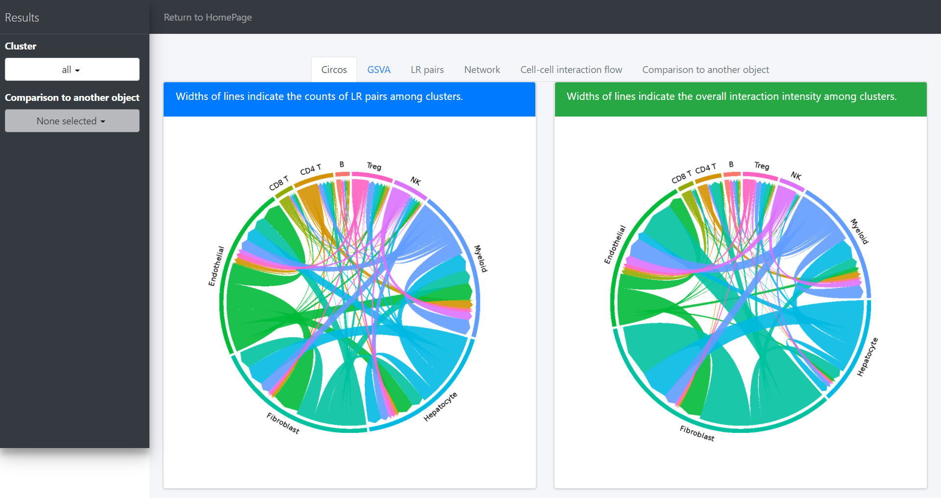
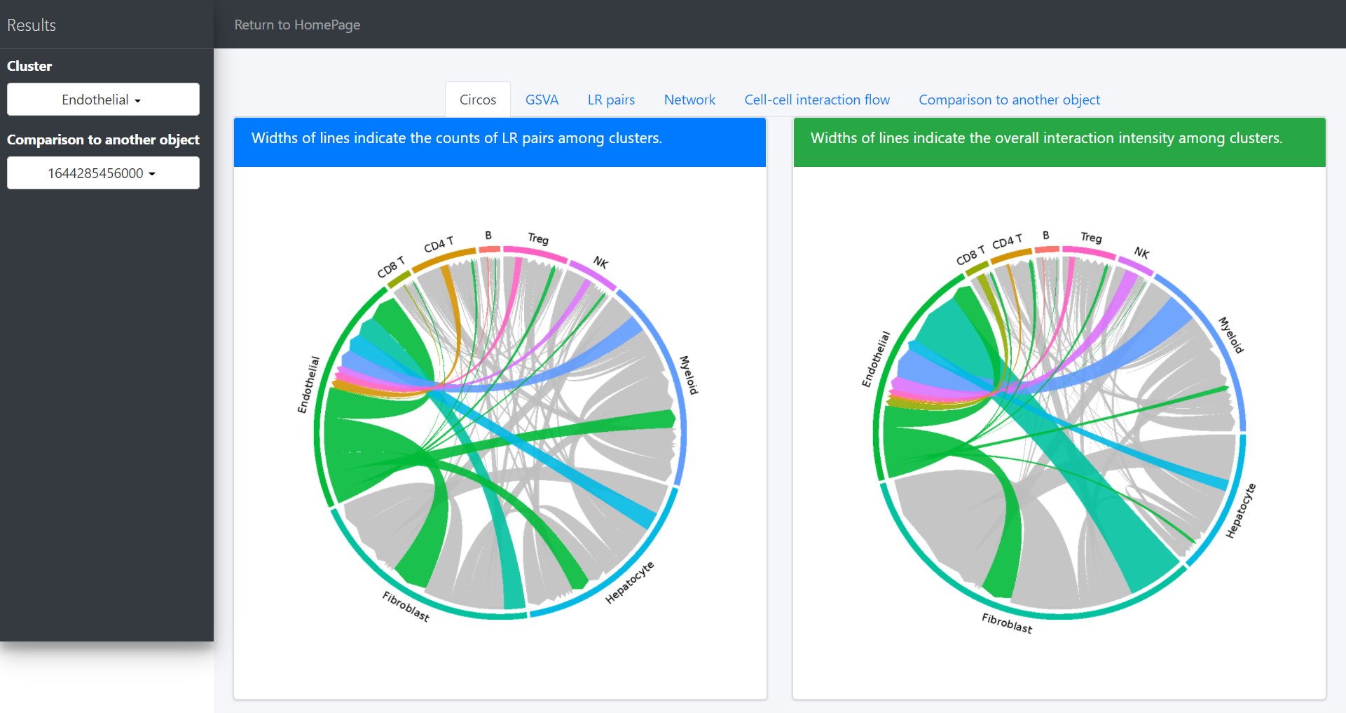
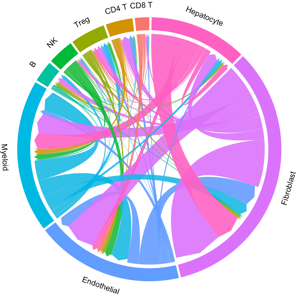
Then you can visualize the interaction through a circos plot:

# Plot interaction for all cluster
circosPlot(object = tumor.obj)

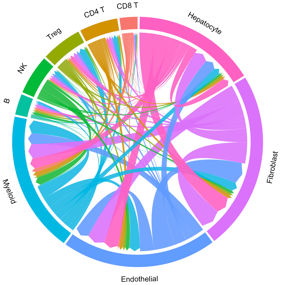
In the above circos plot, the directions of lines indicate the associations from ligands to receptors, and the widths of lines indicate the counts of LR pairs among clusters.

# Plot interaction for all cluster
circosPlot(object = tumor.obj)

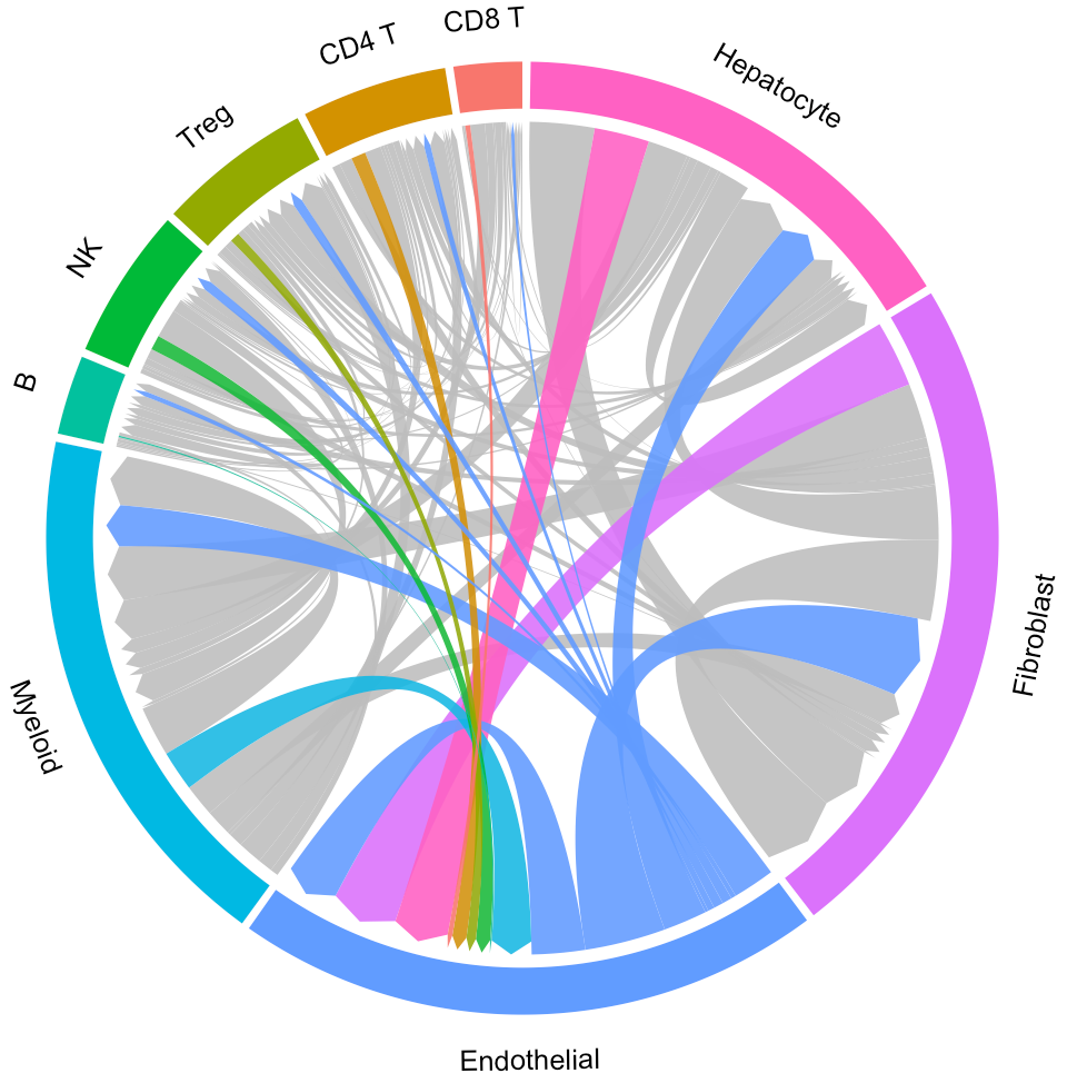
Now the widths of lines indicate the overall interaction intensity among clusters.

# Highlight the interaction of specific cluster
# Here we take the endothelial cell as an example
ident = 'Endothelial'
circosPlot(object = tumor.obj, ident = ident)

For a specific cluster of interest, CommPath provides function findLigand (findReceptor) to find the upstream (downstream) cluster and the corresponding ligand (receptor) for specific cluster and receptor (ligand):

# For the selected cluster and selected receptor, find the upstream cluster
select.ident = 'Endothelial'
select.receptor = 'ACKR1'

ident.up.dat <- findLigand(object = tumor.obj, 
    select.ident = select.ident, 
    select.receptor = select.receptor)
head(ident.up.dat)

# For the selected cluster and selected ligand, find the downstream cluster
select.ident = 'Endothelial'
select.ligand = 'CXCL12'

ident.down.dat <- findReceptor(object = tumor.obj, 
    select.ident = select.ident, 
    select.ligand = select.ligand)
head(ident.down.dat)

There are 7 columns stored in the variable ident.up.dat/ident.down.dat:
Columns Cell.From, Cell.To, Ligand, Receptor show the upstream and dowstream clusters and the specific ligands and receptors in the LR associations;
Columns Log2FC.LR, P.val.LR, P.val.adj.LR show the interaction intensity (measured by the product of Log2FCs of ligands and receptors)and the corresponding original and adjusted p value for hypothesis test of one pair of LR.

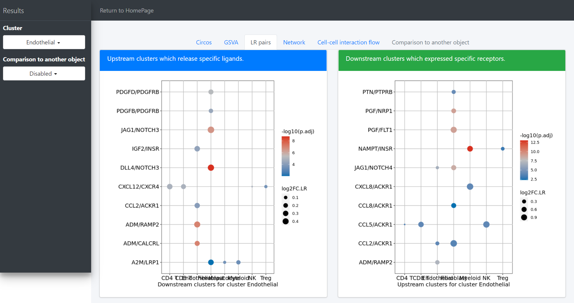
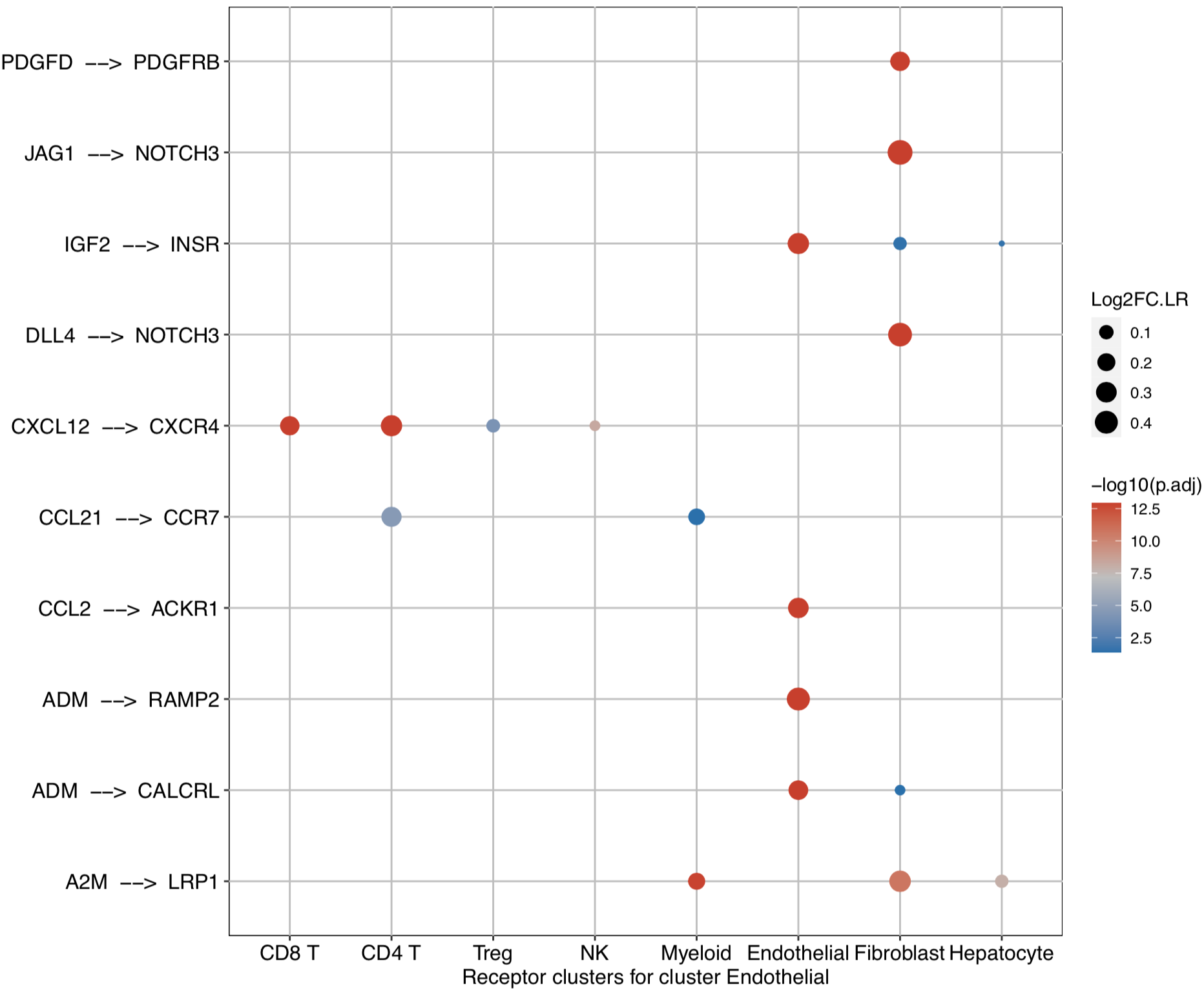
CommPath also provides dot plots to investigate its upstream clusters which release specific ligands and its downstream clusters which expressed specific receptors:

# Investigate the upstream clusters which release specific ligands to the interested cluster
dotPlot(object = tumor.obj, receptor.ident = ident)

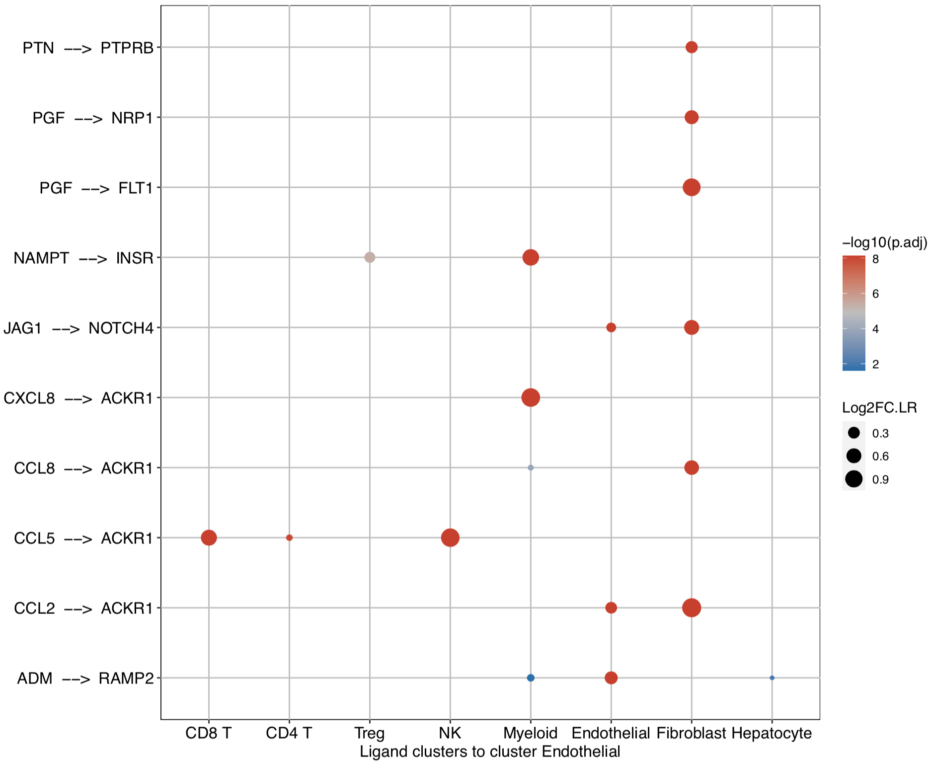
# Investigate the downstream clusters which expressed specific receptors for the interested cluster
dotPlot(object = tumor.obj, ligand.ident = ident)

Pathway analysis

CommPath conducts pathway analysis to identify signaling pathways involving the marker ligands and receptors for each cluster.

# Find pathways in which genesets show overlap with the marker ligands and receptors in the example dataset
# CommPath provides pathway annotations from KEGG pathways, WikiPathways, reactome pathways, and GO terms
tumor.obj <- findLRpath(object = tumor.obj, category = 'kegg')

Now genesets showing overlap with the marker ligands and receptors are stored in tumor.obj@interact[[‘pathwayLR’]]. Then we score the pathways to measure the activation levels for each pathway in each cell.

# Compute pathway activation score by the gsva algorithm or an average manner
# For more information about gsva algorithm, see the GSVA package
tumor.obj <- scorePath(object = tumor.obj, method = 'gsva', min.size = 10, parallel.sz = 4)

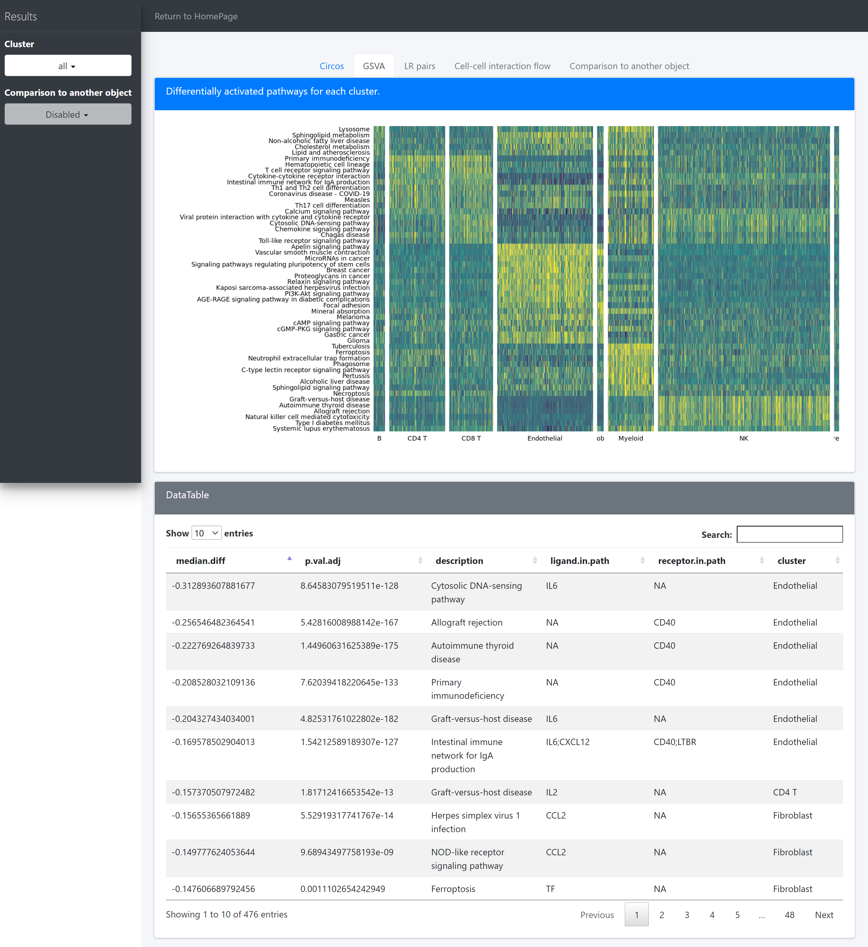
After that CommPath provide diffAllPath to perform pathway differential activation analysis for cells in each identity class and find the receptor and ligand in the pathway:

# get significantly up-regulated pathways in each identity class
acti.path.dat <- diffAllPath(object = tumor.obj, only.posi = TRUE, only.sig = TRUE)
head(acti.path.dat)

There are several columns stored in the variable acti.path.dat:
Columns mean.diff, mean.1, mean.2, t, df, p.val, p.val.adj show the statistic result; description shows the name of pathway;
Columns cell.up and ligand.up show the upstream identity classes which would release specific ligands to interact with the receptors from the current identity class;
Column receptor.in.path shows the marker receptors expressed by the current identity class and these receptors are included in the current pathway;
Column ligand.in.path shows the marker ligands released by the current identity class and these ligands are also included in the current pathway.

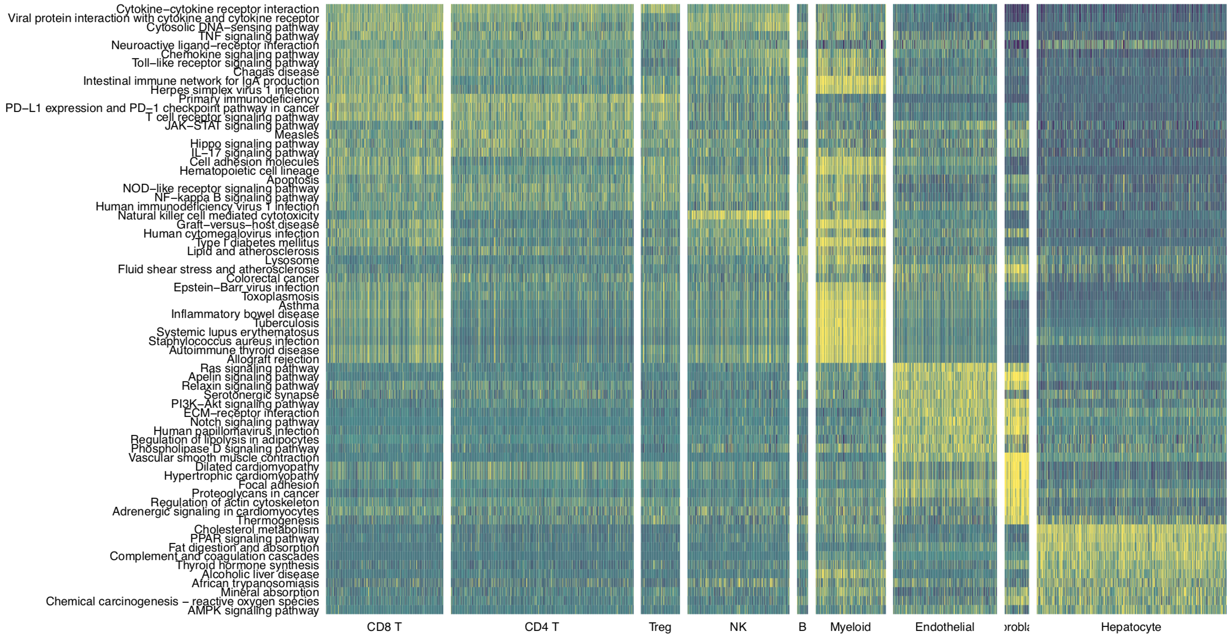
Then we use pathHeatmap to plot a heatmap of those differentially activated pathways for each cluster to display the highly variable pathways:

pathHeatmap(object = tumor.obj,
       acti.path.dat = acti.path.dat,
       top.n.pathway = 10,
       sort = "p.val.adj")

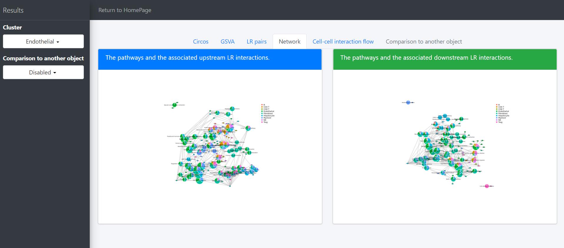
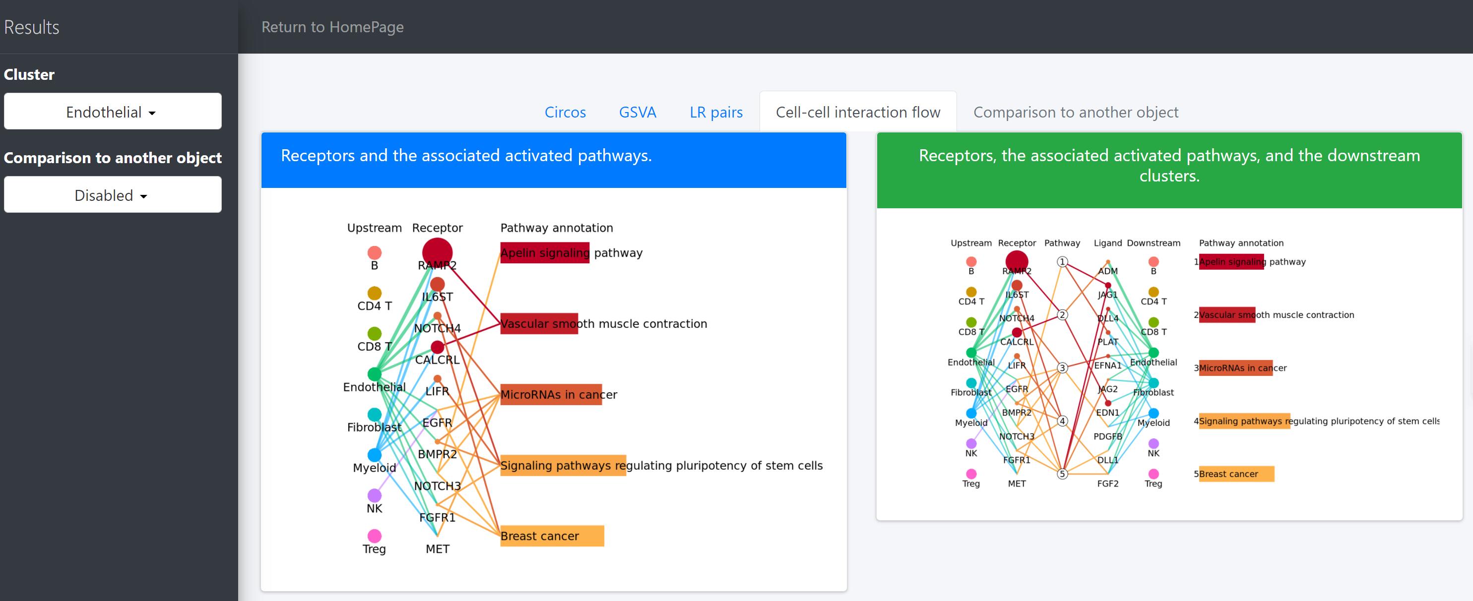
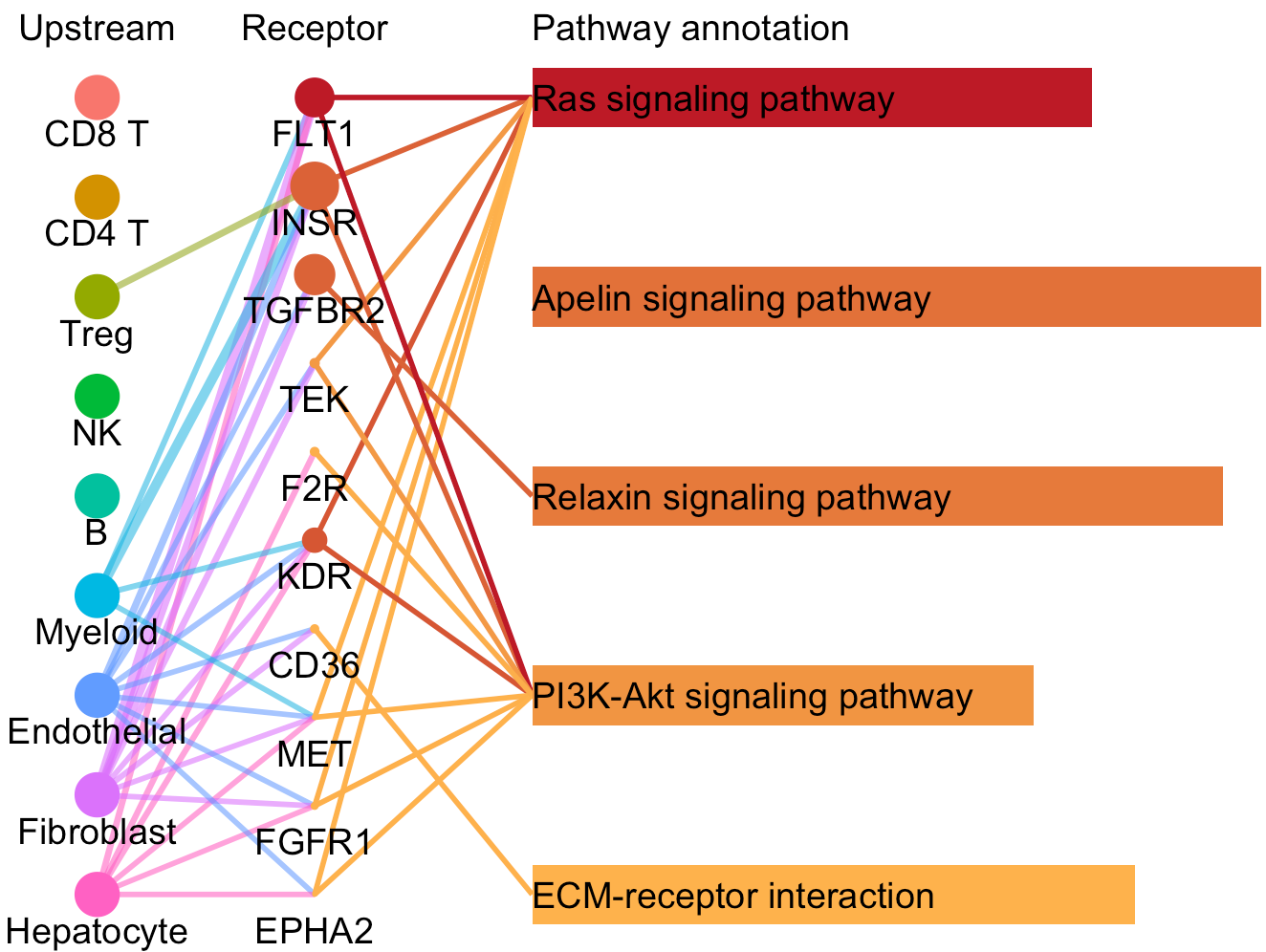
Cell-cell interaction flow via pathways

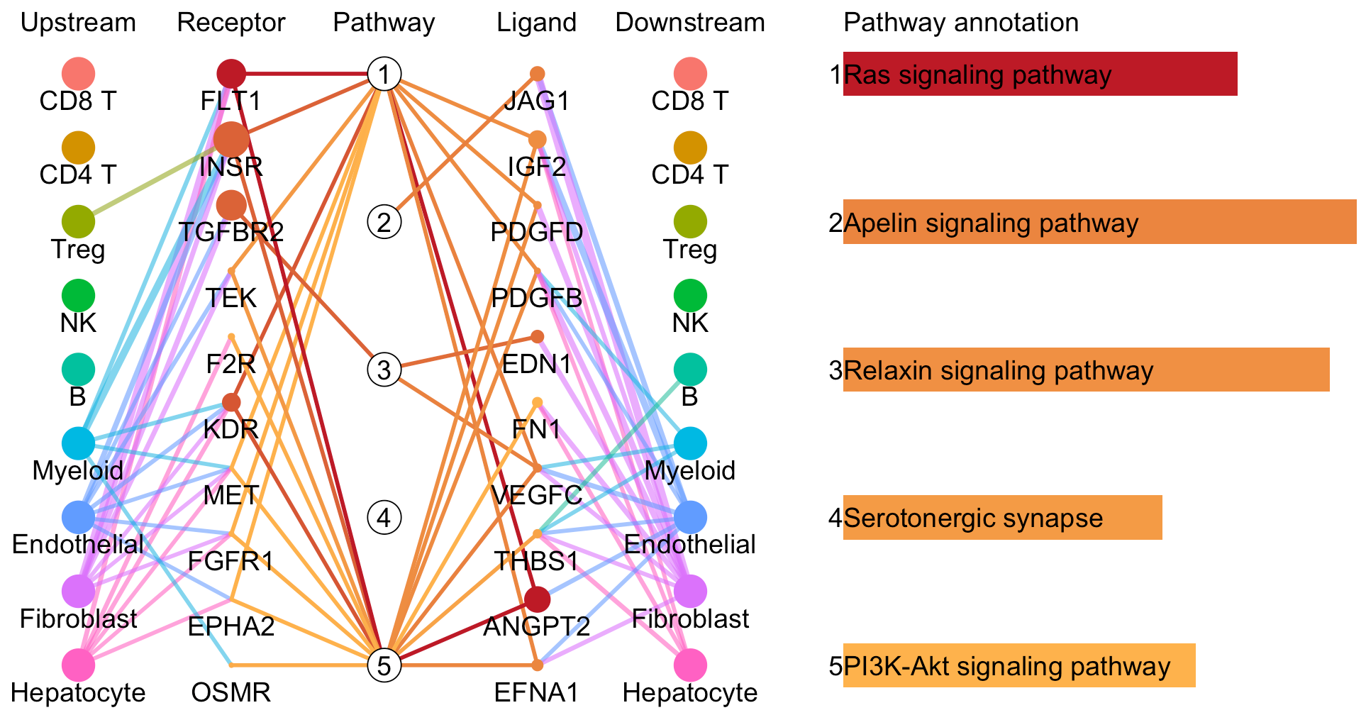
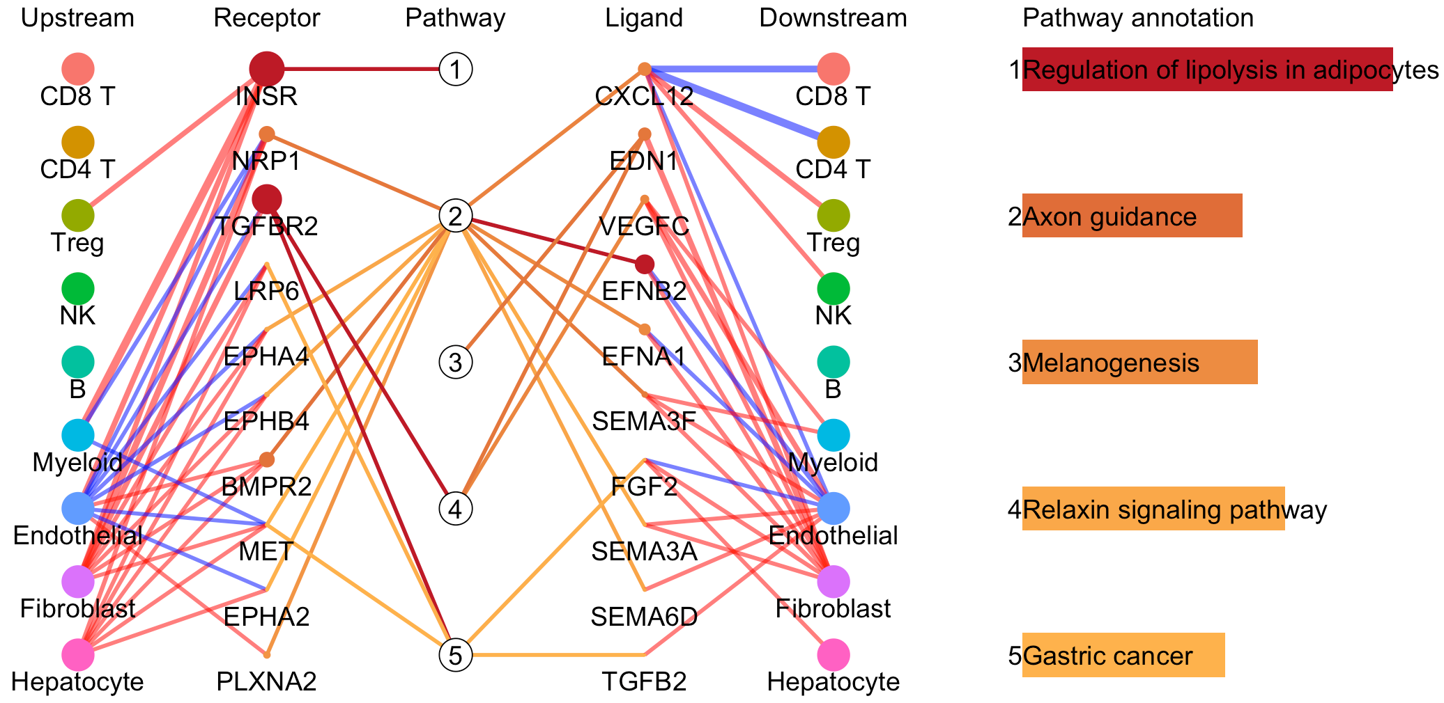
For a specific cell cluster, which here we name it as B for demonstration, CommPath identify the upstream cluster A sending signals to B, the downstream cluster C receiving signals from B, and the significantly activated pathways in B to mediate the A-B-C communication flow. More exactly, through LR and pathways analysis described above, CommPath is able to identify LR pairs between A and B, LR pairs between B and C, and pathways activated in B. Then CommPath screens for pathways in B which involve both the receptors to interact with A and ligands to interact with C.

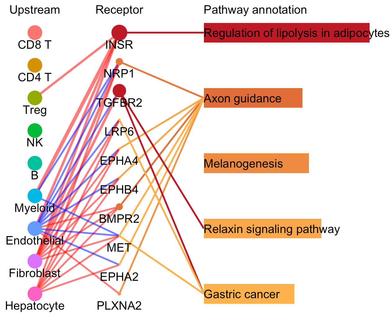
# Identification and visualization of the identified pathways
# Plot to identify receptors and the associated activated pathways for a specific cluster
select.ident = 'Endothelial'
pathPlot(object = tumor.obj, 
    select.ident = select.ident, 
    acti.path.dat = acti.path.dat)

# Plot to identify receptors, the associated activated pathways, and the downstream clusters
pathInterPlot(object = tumor.obj, 
    select.ident = select.ident, 
    acti.path.dat = acti.path.dat)

Compare cell-cell interactions between two conditions

CommPath also provide useful utilities to compare cell-cell interactions between two conditions such as disease and control. Here we, for example, used CommPath to compare the cell-cell interactions between cells from HCC tumor and normal tissues. The example data from normal tissues are also available in figshare.

# load(url("https://figshare.com/ndownloader/files/33926129"))
load("path_to_download/HCC.normal.3k.RData")

We have pre-created the CommPath object for the normal samples following the above steps. This dataset consists of 3 varibles:
normal.expr : expression matrix for cells from normal tissues;
normal.label : indentity lables for cells from normal tissues;
normal.obj : CommPath object created from normal.expr and normal.label, and processed by CommPath steps described above.

To compare 2 CommPath object, we shall first identify the differentially expressed ligands and receptors, and differentially activated pathways between the same cluster of cells in the two object.

# Take endothelial cells as example
# Identification of differentially expressed ligands and receptors 
diff.marker.dat <- diffCommPathMarker(object.1 = tumor.obj, object.2 = normal.obj, select.ident = 'Endothelial')

# Identification of differentially activated pathways 
diff.path.dat <- diffCommPathPath(object.1 = tumor.obj, object.2 = normal.obj, select.ident = 'Endothelial', parallel.sz = 4)

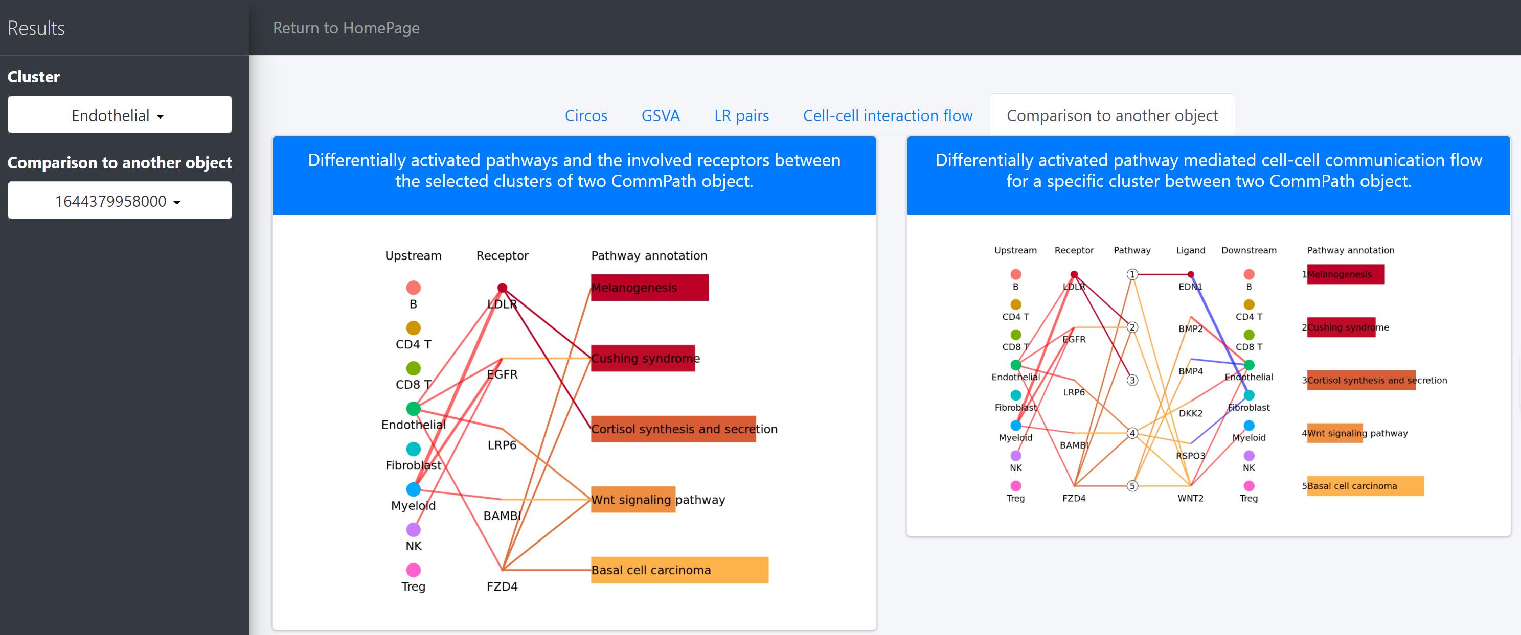
Then we compare the differentially activated pathways and the cell-cell communication flow mediated by those pathways.

# To compare differentially activated pathways and the involved receptors between the selected clusters of two CommPath object
pathPlot.compare(object.1 = tumor.obj, object.2 = normal.obj, select.ident = 'Endothelial', diff.marker.dat = diff.marker.dat, diff.path.dat = diff.path.dat)

# To compare the pathway mediated cell-cell communication flow for a specific cluster between 2 CommPath object
pathInterPlot.compare(object.1 = tumor.obj, object.2 = normal.obj, select.ident = 'Endothelial', diff.marker.dat = diff.marker.dat, diff.path.dat = diff.path.dat)

---

sessionInfo()

R version 4.0.3 (2020-10-10)
Platform: x86_64-conda-linux-gnu (64-bit)
Running under: CentOS Linux 7 (Core)

Matrix products: default
BLAS/LAPACK: /home/luh/miniconda3/envs/seurat4/lib/libopenblasp-r0.3.17.so

locale:
 [1] LC_CTYPE=zh_CN.UTF-8       LC_NUMERIC=C              
 [3] LC_TIME=zh_CN.UTF-8        LC_COLLATE=zh_CN.UTF-8    
 [5] LC_MONETARY=zh_CN.UTF-8    LC_MESSAGES=zh_CN.UTF-8   
 [7] LC_PAPER=zh_CN.UTF-8       LC_NAME=C                 
 [9] LC_ADDRESS=C               LC_TELEPHONE=C            
[11] LC_MEASUREMENT=zh_CN.UTF-8 LC_IDENTIFICATION=C       

attached base packages:
[1] stats     graphics  grDevices utils     datasets  methods   base     

other attached packages:
[1] GSVA_1.38.2     ggplot2_3.3.5   dplyr_1.0.7     reshape2_1.4.4 
[5] circlize_0.4.13 CommPath_0.1.0 

loaded via a namespace (and not attached):
 [1] Rcpp_1.0.7                  lattice_0.20-44            
 [3] digest_0.6.27               assertthat_0.2.1           
 [5] utf8_1.2.2                  R6_2.5.1                   
 [7] GenomeInfoDb_1.26.7         plyr_1.8.6                 
 [9] stats4_4.0.3                RSQLite_2.2.8              
[11] httr_1.4.2                  pillar_1.6.2               
[13] zlibbioc_1.36.0             GlobalOptions_0.1.2        
[15] rlang_0.4.11                annotate_1.68.0            
[17] blob_1.2.2                  S4Vectors_0.28.1           
[19] Matrix_1.3-4                labeling_0.4.2             
[21] BiocParallel_1.24.1         stringr_1.4.0              
[23] RCurl_1.98-1.4              bit_4.0.4                  
[25] munsell_0.5.0               DelayedArray_0.16.3        
[27] compiler_4.0.3              pkgconfig_2.0.3            
[29] BiocGenerics_0.36.1         shape_1.4.6                
[31] tidyselect_1.1.1            SummarizedExperiment_1.20.0
[33] tibble_3.1.3                GenomeInfoDbData_1.2.4     
[35] IRanges_2.24.1              matrixStats_0.60.1         
[37] XML_3.99-0.7                fansi_0.5.0                
[39] crayon_1.4.1                withr_2.4.2                
[41] bitops_1.0-7                grid_4.0.3                 
[43] xtable_1.8-4                GSEABase_1.52.1            
[45] gtable_0.3.0                lifecycle_1.0.0            
[47] DBI_1.1.1                   magrittr_2.0.1             
[49] scales_1.1.1                graph_1.68.0               
[51] stringi_1.7.4               cachem_1.0.6               
[53] farver_2.1.0                XVector_0.30.0             
[55] ellipsis_0.3.2              generics_0.1.0             
[57] vctrs_0.3.8                 tools_4.0.3                
[59] bit64_4.0.5                 Biobase_2.50.0             
[61] glue_1.4.2                  purrr_0.3.4                
[63] MatrixGenerics_1.2.1        parallel_4.0.3             
[65] fastmap_1.1.0               AnnotationDbi_1.52.0       
[67] colorspace_2.0-2            GenomicRanges_1.42.0       
[69] memoise_2.0.0             

2022.2.22

• Add Google Analytics.
• Fix errors when submit a new task with a new file.

---

2022.2.9

• Add annotations for each plot.
• Change appname to CommPath.
• Remove Cluster2 in the result page.
• Fix label errors for comparison-object.

---

2022.2.8

• Fix width-height imbalance.

---

2022.2.7

• On line.

A Single-Cell Atlas of the Multicellular Ecosystem of Primary and Metastatic Hepatocellular Carcinoma

SUMMARY

Hepatocellular carcinoma (HCC) represents a paradigm of the relation between tumor microenvironment (TME) and tumor development. Here, we generated > 70,000 single-cell transcriptomes for 10 HCC patients from four relevant sites: primary tumor, portal vein tumor thrombus (PVTT), metastatic lymph node and non-tumor liver. We discovered a cluster of antitumor central memory T (TCM) cells enriched in intratumoral tertiary lymphoid structures (TLSs) of HCC. We found chronic HBV/HCV infection increases the infiltration of CD8+ T cells in tumors but aggravates the exhaustion of tumor-infiltrating lymphocytes. We identified CD11b+ macrophages to be terminally differentiated tumor-associated macrophages (TAMs) and two distinct differentiation trajectories are related to their accumulation. We further demonstrated CD11b+ TAMs promote HCC cells invasion and migration, and angiogenesis. Our data also revealed the heterogeneous population of malignant hepatocytes and their potential multifaceted roles in shaping the immune microenvironment of HCC. Finally, we identified seven TME subtypes of HCC that can predict patient prognosis. Collectively, this large-scale, single-cell atlas deepens our understanding of the ecosystem in primary and metastatic HCCs, might facilitating the development of new immune therapy strategies for this malignancy.

Droplet-based scRNA-seq and gene expression quantification

Single-cell suspensions were converted to barcoded scRNA-seq libraries by using the Chromium Single Cell 3’ Library, Gel Bead & Multiplex Kit and Chip Kit (10x Genomics), aiming for an estimated 5,000 cells per library and following the manufacturer’s instructions. Samples were processed using kits pertaining to V2 barcoding chemistry of 10x Genomics. Single samples are always processed in a single well of a PCR plate, allowing all cells from a sample to be treated with the same master mix and in the same reaction vessel. For each patient, all samples (NTL, PT, PVTT and MLN) were processed in parallel in the same thermal cycler. The generated scRNA-seq libraries were sequenced on a NovaSeq sequencer (Illumina). The Cell Ranger software (version 2.2.0; 10x Genomics) was used to perform sample demultiplexing, barcode processing and single-cell 3’ counting. Cell Ranger’s mkfastq function was used to demultiplex raw base call files from the sequencer, into sample-specific fastq files. Afterward, fastq files for each sample were processed with Cell Ranger’s count function, which was used to align reads to human genome (build hg38) and quantify gene expression levels in single cells.

Quality control and batch correction

To filter out low-quality cells and doublets (two cells encapsulated in a single droplet), for each sample, cells were removed that had either fewer than 200 unique molecular identifiers (UMIs), over 8,000 or below 200 expressed genes. To filter out dead or dying cells, cells were further removed that had over 10% UMIs derived from mitochondrial genome. This resulted in a total of 71,915 high-quality single-cell transcriptomes in all samples.

To further merge samples across tissues and patients, we run a canonical correlation analysis (CCA) for batch correction using the RunMultiCCA function in R package Seurat v2. To calculate canonical correlation vectors (CCVs), variably expressed genes were selected for each sample as having a normalized expression between 0.125 and 3, and a quantile-normalized variance exceeding 0.5, and then combined across all samples. The resulting 2,773 non-redundant variable genes were summarized by CCA, and the first 15 CCVs were aligned to combine raw gene expression matrices generated per sample. The aligned CCVs were also used for tSNE dimensionality reduction using the RunTSNE function in Seurat.

Cell clustering

For cell clustering, we used the FindClusters function in Seurat v2 that implements shared nearest neighbor (SNN) modularity optimization-based clustering algorithm on 30 aligned CCVs with resolution 1–4, leading to 26–61 clusters. A resolution of 3 was chosen for the analysis and a final of 53 clusters were obtained.

Brief introduction

RegVar is a deep neural network-based computational server for prioritizing tissue-specific regulatory impact of human noncoding SNPs on their potential target genes. RegVar integrates the sequential, epigenetic and evolutionary conservation profiles of SNPs and their potential target genes in 17 human tissues, and give tissue-specific predictions of regulatory probabilities of the provided SNPs on provided genes.

Input

Upload a file containing a list of SNPs and genes

A text file containing a list of SNP IDs and their possible target genes is required to be uploaded to the server for batch analysis.

The result will be generated based on all pairwise combinations of SNPs and genes. SNPs and genes lacking annotations are excluded and pairs of SNPs and genes that are located on different chromosomes are removed. The remaining pairs are referred to as valid pairs and RegVar would accept no more than 10,000 valid pairs.
Click here to see an example file

Or type SNP ID(s) and gene(s) in the corresponding search boxes

SNP ID(s) (indels are currently not supported) and their possible target gene(s) are accepted as input in the SNP and Gene search box, respectively. Multiple SNP IDs or genes should be delimited by commas, spaces or tabs, and if so, the result will be generated based on all pairwise combinations of SNPs and genes.

Output

All results will be listed in the result page, including the basic information of your query data (the positions of the input SNPs and TSSs of genes and the genomic distance between them, in GRCh37/hg19 genome coordinates) (positions of TSSs are annotated from GTEx eGene list, v7 release), and the regulatory probabilities calculated by RegVar.

Raw probability scores come straight from the tissue-specific model, and are interpretable as the extent to which the SNP is likely to have an effect on the regulation of the corresponding gene in your selected tissue.

A result file containing the same information will be sent to your email address, if you have it input.

Model selection

The RegVar website computes RegVar scores based on the DHS-filtered models trained on GTEx datasets. Besides, We also provide the scripts to train non-DHS-filtered models (or full models) on GTEx datasets and to train pathogenic RegVar models on HGMD dataset. Click the following download link for more information.

Software download

The datasets and source code to run RegVar locally are freely available at the download page.

All data from 3dsnp including high-order modified predictions can be accessed through FTP.

You could also click links in the following table.

PS: If you have any questions or would like to access additional data, please leave a message.

Data	Format	Link
dbSNP154	Vcf	example: chr1
HGSVC2	Vcf	pangenie_merged_bi_nosnvs.integrated_callset.hg19
dbSNP153	BigBed	dbSnp153Common.bb
Gene annotations	GFF	GCF_000001405.25_GRCh37.p13_genomic
Gene annotations	RefSeq	ncbiRefSeq
Assembly	Fasta	hg19.fa
ENCODE	BigWig	example: Gm12878 H3k27ac
RepeatMasker	BigBed	repeats
Fixation index	Bed	example: chr1 AMR
xp-NSL	Bed	example: chr1 AMR
ClinVar	BigBed	clinvarCnv clinvarMain
ClinGen	BigBed	clinGenHaplo clinGenTriplo clinGenGeneDisease
scATAC-fetal	BigWig	example: thymus_vascular_endothelial_cells
HiC loops	loop	raw: Ventricle_Right mod: Ventricle_Right target: chr17-42337882-DEL-540 Ventricle_Right